3.6. Vignette for analyzing and plotting isoform Switching for Kinnex Full Length

The isoformSwitchAnalyzeR is an R package developed to enable statistical identification of isoform switching and alternative isoform usage. This vignette is based on the isoformAnlayzeR tutorial provided

We would analyze the bulk samples with this vignette here.

Module to install packages

Setting the environment:

  #{r}
 install_if_missing <- function(packages) {
 if (length(setdiff(packages, rownames(installed.packages()))) > 0) {
     install.packages(setdiff(packages, rownames(installed.packages())))
 }
}

Install tidyverse, IsoformSwitchAnalyzeR and edgeR

#{r}
install_if_missing(c('tidyverse','stringr','dplyr','edgeR','ggrepel'))
if (!require("BiocManager", quietly = TRUE))
 install.packages("BiocManager")
 BiocManager::install(c("IsoformSwitchAnalyzeR","edgeR", "limma", "DESeq2", "ctc", "Biobase", "gplots", "ape", "argparse","dplyr"))

Importing libraraies:

#{r}
set.seed(2023)
library(tidyverse)
library(IsoformSwitchAnalyzeR)
library(edgeR)
library(dplyr)
packageVersion('IsoformSwitchAnalyzeR')
options(warn=-1)

Set working dir:

#{r}
pdir='../Kinnex_bulk/'
setwd(pdir)
counts = read_tsv(file.path(pdir, "isoquant_counts_combined_wRefids.tsv")) %>% as.data.frame()

exploring counts matrix: .. code:: bash

#{r} colnames(counts) length(counts$isoform_id) length(unique(counts$isoform_id)) head(counts$isoform_id,3)

Reading in gtf

#{r}
gtf = read_tsv(file.path(pdir,'stringtie_merged.wRefIds.gtf'), skip = 5, col_names = F) %>% filter(X3 == 'transcript')
##"; transcript_id " "MSTRG.5.2^ENSG00000228794.11^ENST00000445118.7^j"
head(str_split_fixed(gtf$X9, '\\"',5) [,4],5)
transcript_in_db = str_split_fixed(gtf$X9, '\\"',5) [,4]
counts$isoform_id[!(counts$isoform_id %in% transcript_in_db)]
counts2 = as_tibble(transcript_in_db) %>% left_join(as_tibble(counts), c('value' = 'isoform_id'))
counts2[is.na(counts2)] = 0
colnames(counts2) = c('isoform_id', colnames(counts2)[2:length(colnames(counts2))])
counts = as.data.frame(counts2)

Computes counts per million (CPM) or reads per kilobase per million (RPKM) values

#{r}
cpm <- cpm(counts[,-1], log=FALSE)
abundance = as.tibble(cbind(isoform_id = counts[,1],as.tibble(cpm)))
colnames(abundance)[-1][-1]

Creating Design object

#{r}
myDesign <- data.frame(
 sampleID = colnames(abundance)[-1][-1],
 condition = c('wt','wt','wt','mut','mut','mut')
 )
 myDesign

importRdata function

Creates SwitchAnalyzeRlist From Standard R Objects isoformNtFasta obtained by running Gffread on the merged assembly as below: gffread stringtie_merged.wRefIds.gtf -g refs/GRCh38_no_alt.fa -w bulk_kinnex_stringtie_merged.wRefIds.fasta

#{r}
aSwitchList <- importRdata(
 isoformCountMatrix   = counts,
 isoformRepExpression = abundance,
 designMatrix         = myDesign,
 isoformExonAnnoation = file.path(pdir, "stringtie_merged.wRefIds.gtf"),
 isoformNtFasta       = file.path(pdir,"bulk_kinnex_stringtie_merged.wRefIds.fasta"),
 showProgress = FALSE
 )

Terminal Output:

Step 1 of 10: Checking data… Step 2 of 10: Obtaining annotation… importing GTF (this may take a while)… Warning: No CDS annotation was found in the GTF files meaning ORFs could not be annotated. (But ORFs can still be predicted with the analyzeORF() function)Warning: The annotation and quantification (count/abundance matrix and isoform annotation) Seem to be slightly different. Specifically: 1 isoforms were only found in the annotation

Please make sure this is on purpouse since differences will cause inaccurate quantification and thereby skew all analysis.

If you have quantified with Salmon this could be normal since it as default only keep one copy of identical sequnces (can be prevented using the –keepDuplicates option) We strongly encurage you to go back and figure out why this is the case.

3 ( 0.01%) isoforms were removed since they were not expressed in any samples. Step 3 of 10: Fixing StringTie gene annoation problems… There were no need to rescue any annotation Step 4 of 10: Calculating expression estimates from count data… Skipped as user supplied expression via the “isoformRepExpression” argument… Step 5 of 10: Testing for unwanted effects… Added 1 batch/covariates to the design matrix Step 6 of 10: Batch correcting expression estimates… Step 7 of 10: Extracting data from each condition… Step 8 of 10: Making comparisons… Step 9 of 10: Making switchAnalyzeRlist object… Step 10 of 10: Guestimating differential usage…

## comparison estimated_genes_with_dtu <chr> <chr> mut vs wt 42 - 70

Pre-filtering switchObject on threholds

#default values: #dIF differential Isoform Usage cutoff (IF isoform fraction) required to consider an isoform switching = 0.1 10% #https://rdrr.io/bioc/IsoformSwitchAnalyzeR/man/preFilter.html

#{r}
aSwitchList <- preFilter(
 switchAnalyzeRlist = aSwitchList,
 IFcutoff=0.01,
 acceptedGeneBiotype = NULL,
 acceptedIsoformClassCode = NULL,
 removeSingleIsoformGenes = TRUE,
 reduceToSwitchingGenes=FALSE,
 reduceFurtherToGenesWithConsequencePotential = FALSE,
 onlySigIsoforms = FALSE,
 keepIsoformInAllConditions=FALSE,
 alpha=0.05,
 dIFcutoff = 0.1,
 quiet=FALSE
 )

Terminal Out: filtering removed 24317 ( 94.07% of ) transcripts. There is now 1534 isoforms left.

Analyze ORFs

#{r}
### 2.2
 aSwitchList = analyzeORF(
 aSwitchList,
 genomeObject = NULL,
 minORFlength=100,
 orfMethod = "longest",
 cds = NULL,
 PTCDistance = 25,
 startCodons="ATG",
 stopCodons=c("TAA", "TAG", "TGA"),
 showProgress=TRUE,
 quiet=FALSE
 )

Terminal Out: Step 1 of 3 : Extracting transcript sequences… Step 2 of 3 : Locating potential ORFs… 100% Step 3 of 3 : Scanning for PTCs… 1532 putative ORFs were identified, analyzed and added. Done

#{r}
group <- factor(aSwitchList$designMatrix$condition)
 y <- DGEList(counts=aSwitchList$isoformCountMatrix,group=group)
 y <- normLibSizes(y)
 design <- model.matrix(~group)
 y <- estimateDisp(y, design)
 y <- estimateTagwiseDisp(y)
 et <- exactTest(y, pair = c('wt','mut'))
 res1 = mutate(topTags(et, n = nrow(et$table))$table, condition_1 = 'wt', condition_2 = 'mut')
 res = rbind(res1)
 res = mutate(res, condition_join = paste(res$condition_1, res$condition_2, res$isoform_id, sep = '_'))

Isoform analyze Part1:

https://bioconductor.org/packages/devel/bioc/manuals/IsoformSwitchAnalyzeR/man/IsoformSwitchAnalyzeR.pdf

#{r}
### 2.3
 aSwitchList_part1 <- isoformSwitchAnalysisPart1(
     switchAnalyzeRlist   = aSwitchList,
     pathToGTF =  file.path(pdir, "stringtie_merged.wRefIds.gtf") ,
     pathToOutput = file.path(pdir, "isoformSwitchAnalysisR/Output/isoformSwitchAnalysisPart1_results"),
     outputSequences      = TRUE, # change to TRUE whan analyzing your own data
     prepareForWebServers = TRUE,  # change to TRUE if you will use webservers for external sequence analysis
 )
 summary(aSwitchList_part1)
 #saveRDS(aSwitchList_part1, 'aSwitchList.rds')

Terminal Out:

Step 1 of 3 : Detecting isoform switches… Step 3 of 3 : Extracting (and outputting) sequences The ‘removeLongAAseq’ and ‘removeShortAAseq’ arguments: Removed : 0 isoforms. Trimmed : 1 isoforms (to only contain the first 1000 AA) The ‘alsoSplitFastaFile’ caused 1 fasta files, each with a subset of the data, to be created (each named X of Y).

The number of isoform switches found were: The nucleotide and amino acid sequences of these isoforms have been outputted to the supplied directory. These sequences enabling external analysis of protein domians (Pfam), coding potential (CPAT/CPC2) or signal peptides (SignalIP). See ?analyzeCPAT, ?analyzeCPC2, ?analyzePFAM or?analyzeSignalIP (under details) for suggested ways of running these three tools.

#{r}
summary(aSwitchList_part1)

Terminal Out:

This switchAnalyzeRlist list contains: 72 isoforms from 33 genes 1 comparison from 2 conditions (in total 6 samples)

Switching features:

Feature analyzed: [1] “Isoform Switch Identification, ntSequence, ORFs, aaSequence”

Restart point: .. code:: bash

#{r} #aSwitchList_part1 = readRDS(‘aSwitchList.rds’)

#{r}
summary(aSwitchList_part1$isoformCountMatrix)
 dim(aSwitchList_part1$isoformCountMatrix)
 aSwitchList_part1$isoformCountMatrix

 aSwitchList <- aSwitchList_part1
 group <- factor(aSwitchList$designMatrix$condition)
 group

DGEList function

Creates a DGEList object from a table of counts (rows=features, columns=samples), group indicator for each column, library size (optional) and a table of feature annotation (optional).

normLibSizes - The normLibSizes function normalizes the library sizes in such a way to minimize the log-fold changes between the samples for most genes. The default method for computing these scale factors uses a trimmed mean of M-values (TMM) between each pair of samples.

#{r}
y <- DGEList(counts=aSwitchList$isoformCountMatrix,group=group)
y <- normLibSizes(y)

~group
 design <- model.matrix(~group)
 design

estimateDisp: from edgeR package Maximizes the negative binomial likelihood to give the estimate of the common, trended and tagwise dispersions across all tags.

#{r}
estimateDisp(y, design)
y <- estimateDisp(y, design)

estimateTagwiseDisp from edgeR: Estimates tagwise dispersion values by an empirical Bayes method based on weighted conditional maximum likelihood

#{r}
estimateTagwiseDisp(y)
y <- estimateTagwiseDisp(y)

exactTest for edgeR: Compute genewise exact tests for differences in the means between two groups of negative-binomially distributed counts.

#{r}
et <- exactTest(y, pair = c('wt','mut'))
et

res1 = mutate(topTags(et, n = nrow(et$table))$table, condition_1 = 'mut', condition_2 = 'wt')
res = rbind(res1)
res = mutate(res, condition_join = paste(res$condition_1, res$condition_2, res$isoform_id, sep = '_'))
res

Mutating isoformSwitchObject

#{r}
aSwitchList_condition_join = paste(aSwitchList$isoformFeatures$condition_1, aSwitchList$isoformFeatures$condition_2, aSwitchList$isoformFeatures$isoform_id, sep = '_')
aSwitchList$isoformFeatures$iso_p_value = res$PValue[match(aSwitchList_condition_join, res$condition_join)]
aSwitchList$isoformFeatures$iso_q_value = res$FDR[match(aSwitchList_condition_join, res$condition_join)]
aSwitchList$isoformFeatures$iso_significant = res$FDR[match(aSwitchList_condition_join, res$condition_join)] < 0.05
aSwitchList$isoformFeatures$iso_significant[aSwitchList$isoformFeatures$iso_significant == TRUE] = 'yes'
aSwitchList$isoformFeatures$iso_significant[aSwitchList$isoformFeatures$iso_significant == FALSE] = 'no'

#{r}
summary(aSwitchList$isoformFeatures$isoform_switch_q_value)
summary(res$FDR[match(aSwitchList_condition_join, res$condition_join)] < 0.05)
res$FDR[match(aSwitchList_condition_join, res$condition_join)] < 0.05

head(str_split_fixed(aSwitchList$isoformFeatures$isoform_id, '\\^',4))

Getting gene names and gene symbols: .. code:: bash

#{r} library(‘biomaRt’) library(‘devtools’) if(!require(‘annotables’)) { install.packages(‘annotables’) library(‘annotables’) } BiocManager::install(“org.Hs.eg.db”)

#Getting GRCh38 reference: if (!require(“BiocManager”, quietly = TRUE)) install.packages(“BiocManager”)

BiocManager::install(“BSgenome.Hsapiens.NCBI.GRCh38”)

#EnsDb.Hsapiens.v86 reference database: if (!require(“BiocManager”, quietly = TRUE)) install.packages(“BiocManager”)

BiocManager::install(“EnsDb.Hsapiens.v86”)

This function returns a list of BioMart databases hosted by Ensembl. To establish a connection use the useMart function.

#{r}
listEnsembl()
ensmbl <- useEnsembl(biomart = "genes")
ensml_datasets <- listDatasets(ensmbl)

useMart func: Connects to the selected BioMart database and dataset

#{r}
mart = useMart("ensembl")
mart = useMart(biomart="ensembl", dataset="hsapiens_gene_ensembl")

#{r}
attr <- listAttributes(mart)
filters <- listFilters(mart)

Ref Ensmbl Ids in dataset

#{r}
isoformFeatures_wIds <- aSwitchList$isoformFeatures
isoformFeatures_wIds$ref_transcript_id <- str_split_fixed(isoformFeatures_wIds$isoform_id, '\\^',4)[,3]
isoformFeatures_wIds$ref_gene_id <- str_split_fixed(isoformFeatures_wIds$isoform_id, '\\^',4)[,2]

#{r}
refIds <- getBM(attributes = c('ensembl_gene_id_version','ensembl_transcript_id_version',
                  'external_gene_name','external_transcript_name'),
   filters = "ensembl_gene_id_version",
   values = isoformFeatures_wIds$ref_gene_id,
   mart = mart
)

#{r}
refIds <- refIds %>% unique()
refIds
colnames(refIds) = c('gene_id', 'transcript_id', 'gene_name', 'transcript_name')
refIds

#{r}
isoformFeatures_wIds <- left_join(isoformFeatures_wIds %>% dplyr::select(-c("gene_name")),
                  refIds %>%
                  unique(),
        by=c("ref_transcript_id"="transcript_id",
             "ref_gene_id"="gene_id"))

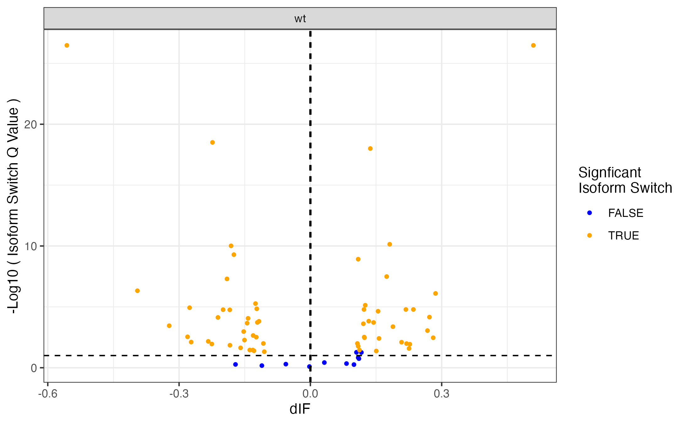
Volcano like plot

#{r}
### Volcano like plot:
 library(ggrepel)

 ggplot(data=isoformFeatures_wIds, aes(x=dIF, y=-log10(isoform_switch_q_value)), label=isoformFeatures_wIds$isoform_id) +
  geom_point(
     aes( color=abs(dIF) > 0.1 & isoform_switch_q_value < 0.05,), # default cutoff
     size=1
 ) +
 geom_hline(yintercept = -log10(0.1), linetype='dashed') + # default cutoff
 geom_vline(xintercept = c(-0.001, 0.001), linetype='dashed') + # default cutoff
 facet_wrap( ~ condition_2) +
 #facet_grid(condition_1 ~ condition_2) + # alternative to facet_wrap if you have overlapping conditions
 scale_color_manual('Signficant\nIsoform Switch', values = c('blue','orange')) +
 labs(x='dIF', y='-Log10 ( Isoform Switch Q Value )') +
 theme_bw()

#{r}
library(ggrepel)

 nbaplot = ggplot(data=isoformFeatures_wIds, aes(x=dIF, y=-log10(isoform_switch_q_value)), label=isoformFeatures_wIds$isoform_id) +
  geom_point(
     aes( color=abs(dIF) > 0.01 & isoform_switch_q_value < 0.05,), # default cutoff
     size=1
 ) +
 geom_hline(yintercept = -log10(0.1), linetype='dashed') + # default cutoff
 geom_vline(xintercept = c(-0.001, 0.001), linetype='dashed') + # default cutoff
 facet_wrap( ~ condition_2) +
 #facet_grid(condition_1 ~ condition_2) + # alternative to facet_wrap if you have overlapping conditions
 scale_color_manual('Signficant\nIsoform Switch', values = c('blue','orange')) +
 labs(x='dIF', y='-Log10 ( Isoform Switch Q Value )') +
 theme_bw()

 nbaplot +
 geom_label_repel(aes(label=ifelse(-log10(isoform_switch_q_value)>0.1,as.character(isoformFeatures_wIds$transcript_name),'')),
               box.padding   = 0.35,
               point.padding = 0.1,
               segment.color = 'grey40')

Switch vs Gene changes

#{r}
ggplot(data=isoformFeatures_wIds, aes(x=gene_log2_fold_change, y=dIF)) +
 geom_point(
     aes( color=abs(dIF) > 0.1 & isoform_switch_q_value < 0.05 ), # default cutoff
     size=1
 ) +
 facet_wrap(~ condition_2) +
 #facet_grid(condition_1 ~ condition_2) + # alternative to facet_wrap if you have overlapping conditions
 geom_hline(yintercept = 0, linetype='dashed') +
 geom_vline(xintercept = 0, linetype='dashed') +
 scale_color_manual('Signficant\nIsoform Switch', values = c('blue','orange')) +
 labs(x='Gene log2 fold change', y='dIF') +
 theme_bw()

Restart point:

#{r}
#saveRDS(aSwitchList_part1, 'aSwitchList.rds')
#aSwitchList_part1 = readRDS('aSwitchList.rds')

isoformSwitchAnalysisPart2 :

adds the results of the external sequence analysis supplied and then analyzes alternative splicing.

Pfam annotations are required, in addition we can provide annotations generated with the tools below. CPC2 Coding Potential Calculator : https://cpc2.gao-lab.org/

Pfam - domain annotation pfam_scan.pl -as -dir isoformSwitchAnalysisPart1_results -fasta isoformSwitchAnalyzeR_isoform_AA_complete.fasta -cpu 4 -e_seq 10.0 -e_dom 10.0 > Pfam_result.txt

IUPred Intrinsically disordered proteins (IDPs) : https://iupred2a.elte.hu/

SignalP Signal peptide and cleavage sites in gram+, gram- and eukaryotic amino acid sequences (signal pipetide at N terminus) : https://services.healthtech.dtu.dk/services/SignalP-5.0/

#{r}
aSwitchList <- analyzePFAM(
 aSwitchList,
 pathToPFAMresultFile = file.path(pdir, "isoformSwitchAnalysisR/Output/Pfam_out.txt"),
 showProgress=TRUE,
 quiet=FALSE

 )

#{r}
 aSwitchList <- isoformSwitchAnalysisPart2(
switchAnalyzeRlist        = aSwitchList,
n                         = 10,    # if plotting was enabled, it would only output the top 10 switches
removeNoncodinORFs        = TRUE,
pathToCPC2resultFile      = file.path(pdir, "isoformSwitchAnalysisR/Output/cpc2output.txt"),
pathToIUPred2AresultFile  = file.path(pdir, "isoformSwitchAnalysisR/Output/iupred2a_out.txt"),
pathToSignalPresultFile   = file.path(pdir, "isoformSwitchAnalysisR/Output/prediction_results.txt"),
pathToDeepTMHMMresultFile = file.path(pdir, "isoformSwitchAnalysisR/Output/TMRs.gff3"),
outputPlots               = TRUE
 )

For DeepLoc annotations, we add a small custom code to format input annotations file:

The input file should have column names in format as below:

#{r}
library(stringr)
deeploc <- read.csv(file.path(pdir, "isoformSwitchAnalysisR/Output/DeepLoc_results.csv"))
deeploc$Protein_ID <- str_replace_all(deeploc$Protein_ID, fixed("_"), "^")
names(deeploc)
names(deeploc) <- gsub("\\.", " ", names(deeploc))
names(deeploc)
write.csv(deeploc,file.path(pdir, "isoformSwitchAnalysisR/Output/DeepLoc_results_wCarets.csv"), row.names = FALSE)

Reading the results in:

#{r}
aSwitchList_wRefIds <- analyzeDeepLoc2(
   switchAnalyzeRlist = aSwitchList_wRefIds,
   pathToDeepLoc2resultFile = file.path(pdir, "isoformSwitchAnalysisR/Output/DeepLoc_results_wCarets.csv"),
   quiet = FALSE
)

Terminal Out: Added subcellular information to 60 (83.33%) transcripts

extracted all switches

#{r}
extractTopSwitches(aSwitchList_wRefIds, filterForConsequences = TRUE, n=10)

analyzeSwitchConsequences: .. code:: bash

#{r} analyzeSwitchConsequences(aSwitchList_wRefIds, consequencesToAnalyze = ‘all’)

Splitting the Long Ids in it’s constituent parts: Renaming Isoform Id by Transcript ID and Gffcompare class codes

#{r}
aSwitchList_wRefIds$isoformFeatures$isoform_id <- paste(str_split_fixed(aSwitchList_wRefIds$isoformFeatures$isoform_id, '\\^',4)[,3],str_split_fixed(aSwitchList_wRefIds$isoformFeatures$isoform_id, '\\^',4)[,4], sep = "_")
aSwitchList_wRefIds$isoformCountMatrix$isoform_id <- paste(str_split_fixed(aSwitchList_wRefIds$isoformCountMatrix$isoform_id, '\\^',4)[,3],str_split_fixed(aSwitchList_wRefIds$isoformCountMatrix$isoform_id, '\\^',4)[,4], sep = "_")
aSwitchList_wRefIds$isoformRepExpression$isoform_id <- paste(str_split_fixed(aSwitchList_wRefIds$isoformRepExpression$isoform_id, '\\^',4)[,3],str_split_fixed(aSwitchList_wRefIds$isoformRepExpression$isoform_id, '\\^',4)[,4], sep = "_")
aSwitchList_wRefIds$isoformRepIF$isoform_id <- paste(str_split_fixed(aSwitchList_wRefIds$isoformRepIF$isoform_id, '\\^',4)[,3],str_split_fixed(aSwitchList_wRefIds$isoformRepIF$isoform_id, '\\^',4)[,4], sep = "_")
aSwitchList_wRefIds$orfAnalysis$isoform_id <- paste(str_split_fixed(aSwitchList_wRefIds$orfAnalysis$isoform_id, '\\^',4)[,3],str_split_fixed(aSwitchList_wRefIds$orfAnalysis$isoform_id , '\\^',4)[,4], sep = "_")
aSwitchList_wRefIds$isoformSwitchAnalysis$isoform_id <- paste(str_split_fixed(aSwitchList_wRefIds$isoformSwitchAnalysis$isoform_id, '\\^',4)[,3],str_split_fixed(aSwitchList_wRefIds$isoformSwitchAnalysis$isoform_id , '\\^',4)[,4], sep = "_")
aSwitchList_wRefIds$topologyAnalysis$isoform_id <- paste(str_split_fixed(aSwitchList_wRefIds$topologyAnalysis$isoform_id, '\\^',4)[,3],str_split_fixed(aSwitchList_wRefIds$topologyAnalysis$isoform_id , '\\^',4)[,4], sep = "_")

plotting “CAPG” out:

#{r}
options(repr.plot.width = 10, repr.plot.height = 5, repr.plot.res = 200)
switchPlot(
   aSwitchList_wRefIds,
   gene = 'CAPG',
   condition1 = 'mutant',
   condition2 = 'wt',
)

plotting “RPS24” out:

  #{r}
   options(repr.plot.width = 10, repr.plot.height = 5, repr.plot.res = 200)
   switchPlot(
     aSwitchList_wRefIds,
     gene = 'RPS24',
     condition1 = 'mutant',
     condition2 = 'wt',
)

plotting “DDX5” out:

  #{r}
   options(repr.plot.width = 10, repr.plot.height = 5, repr.plot.res = 200)
   switchPlot(
     aSwitchList_wRefIds,
     gene = 'DDX5',
     condition1 = 'mutant',
     condition2 = 'wt',
)

plotting “CANX” out:

  #{r}
   options(repr.plot.width = 10, repr.plot.height = 5, repr.plot.res = 200)
   switchPlot(
     aSwitchList_wRefIds,
     gene = 'CANX',
     condition1 = 'mutant',
     condition2 = 'wt',
)

.. image:: ../_images/CANX.png
  :align: center

plotting “FAH” out:

  #{r}
   options(repr.plot.width = 10, repr.plot.height = 5, repr.plot.res = 200)
   switchPlot(
     aSwitchList_wRefIds,
     gene = 'FAH',
     condition1 = 'mutant',
     condition2 = 'wt',
)

plotting “TSEN15” out:

  #{r}
   options(repr.plot.width = 10, repr.plot.height = 5, repr.plot.res = 200)
   switchPlot(
     aSwitchList_wRefIds,
     gene = 'TSEN15',
     condition1 = 'mutant',
     condition2 = 'wt',
)

plotting “NDUFB10” out:

  #{r}
   options(repr.plot.width = 10, repr.plot.height = 5, repr.plot.res = 200)
   switchPlot(
     aSwitchList_wRefIds,
     gene = 'NDUFB10',
     condition1 = 'mutant',
     condition2 = 'wt',
)