3.2 Vignette for Tertiary processing for SC-Kinnex#
This vigentte leverages various parts of the Seurat package and follows along in parts the “Seurat - Guided Clustering Tutorial” The standalone utility scIsoseqUtil.py, developed at MDL, creates sparce matrices from Isoquant Outs namely, transcript_model_reads and transcript_models_gtfs. The script is provided in source repo here.
Creating sparse matrices for use with Seurat#
Setting the environment:
sudo apt install r-base
sudo R -e 'install.packages("BiocManager", repos="http://cran.us.r-project.org")'
sudo R -e 'BiocManager::install("argparse")'
conda create -n scIsoseqUtil
conda activate scIsoseqUtil
conda install bioconda::r-argparse
pip install pysam
# from:
# https://github.com/MethodsDev/scIsoquantMatrixBuilder

wget https://github.com/MethodsDev/kinnex-documentation-external/archive/refs/heads/main.zip

scIsoseqUtil.py --sample_id ${sample_id} \
                --bam ${sample_id}.aligned.sorted.bam \
                --transcript_model_reads ${sample_id}.transcript_model_reads.tsv.gz \
                --transcript_models_gtf ${sample_id}.transcript_models.gtf.gz
Analysing sparse matrices created above#
The code below is an R code, blocks can be copied to Rmd to excute locally:
install_if_missing <- function(packages) {
if (length(setdiff(packages, rownames(installed.packages()))) > 0) {
    install.packages(setdiff(packages, rownames(installed.packages())))
    }
}

install_if_missing(c('tidyverse','stringr','dplyr','edgeR','ggrepel','DESeq2','Seurat','clustermole'))
# {r setup, include=FALSE}
    knitr::opts_chunk$set(echo = TRUE)
    library(tidyverse)
    library(Seurat)
Input counts matrix created above from step1#
#{r}
    data_dir = "scKinnex.genes-sc_matrix_from_isoquant/"
    output_prefix = "scKinnex.genes"
Reading data in using Read10x()#
#{r}
    data = Read10X(data.dir=data_dir,
           gene.column = 1,
           cell.column = 2,
           unique.features = TRUE,
           strip.suffix = FALSE)
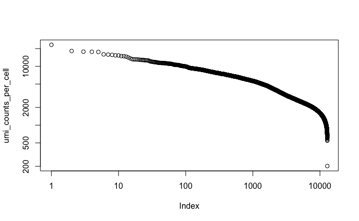
UMI counts per cell:#
#{r}
    umi_counts_per_cell = colSums(data)
sorting:#
#{r}
    umi_counts_per_cell = sort(umi_counts_per_cell, decreasing = T)
plotting :#
#{r}
    plot(umi_counts_per_cell, log='xy')
    ggsave(filename='PBMC_complete_umi_counts_per_cell.png',path=data_dir, plot = last_plot())
Creating seurat object from counts matrix#
#{r}
seurat_obj <- CreateSeuratObject(counts = data, project = "project", min.cells = 3, min.features = 200)
seurat_obj
Output: An object of class Seurat 25943 features across 12851 samples within 1 assay Active assay: RNA (25943 features, 0 variable features) 1 layer present: counts
#{r}
# before filtering
seurat_obj@meta.data %>% summarize(median(nCount_RNA), median(nFeature_RNA))
Terminal Out:
median(nCount_RNA) median(nFeature_RNA) <dbl> <dbl> 2250.01 1087
PercentageFeatureSet - Calculate the percentage of all counts that belong to a given set of features
#{r}
    seurat_obj[["percent.mt"]] <- PercentageFeatureSet(seurat_obj, pattern = "^MT-")
Exploring seurat object:
#{r}
    seurat_obj
    seurat_obj@meta.data %>% head()
UMI counts per cell#
#{r}
seurat_obj@meta.data %>% dplyr::select(nCount_RNA) %>%
arrange(desc(nCount_RNA)) %>%
dplyr::mutate(i=row_number()) %>%
ggplot(aes(x=i, y=nCount_RNA)) + geom_point() + theme_bw() +
scale_y_continuous(trans='log10') +
scale_x_continuous(trans='log10') +
ggtitle("nCount_RNA: UMI counts per cell")

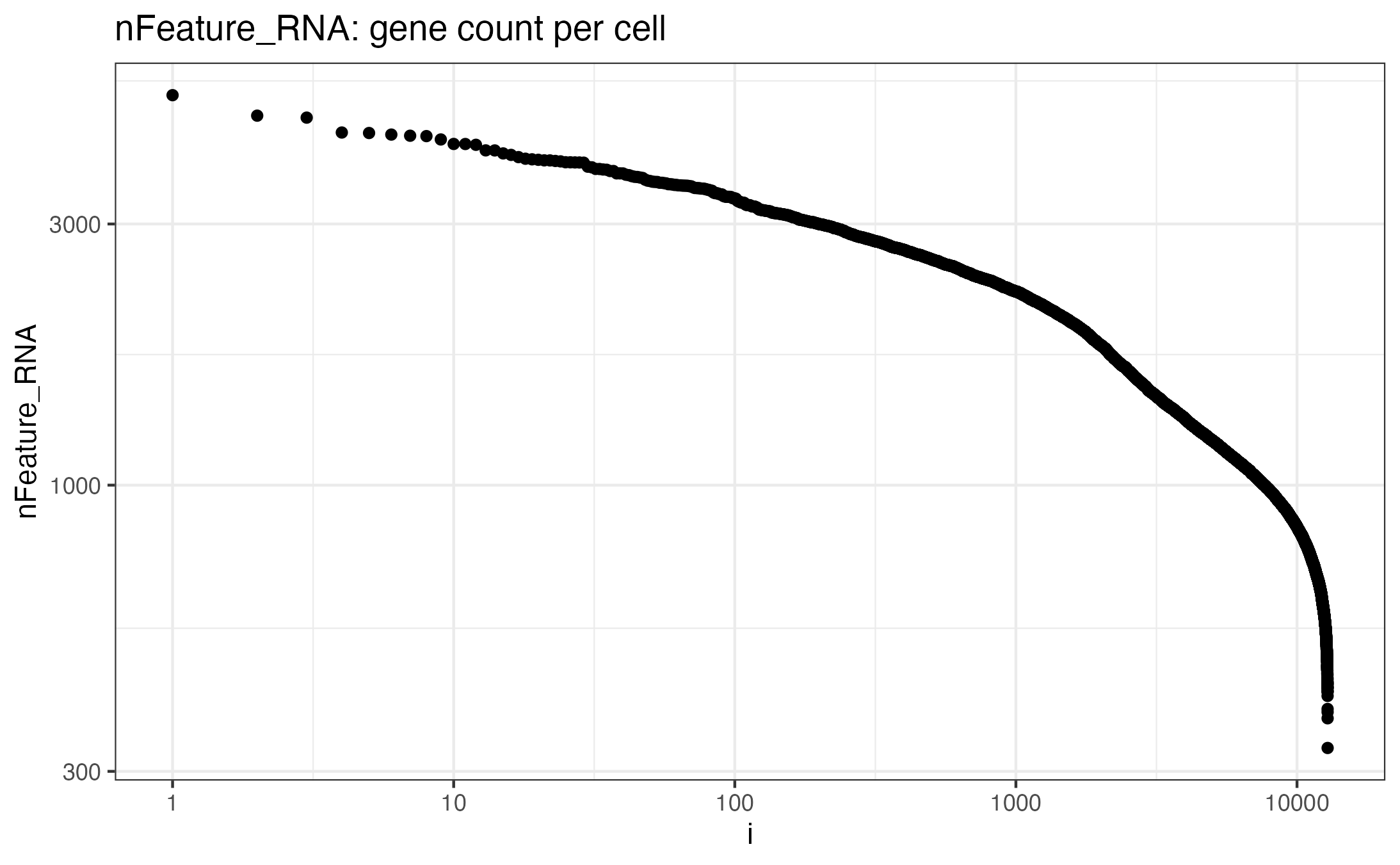
Feature counts per cell:#
#{r}
    seurat_obj@meta.data %>% dplyr::select(nFeature_RNA) %>% arrange(desc(nFeature_RNA)) %>% dplyr::mutate(i=row_number()) %>%
    ggplot(aes(x=i, y=nFeature_RNA)) + geom_point() + theme_bw() +
    scale_y_continuous(trans='log10') +
    scale_x_continuous(trans='log10') +
    ggtitle("nFeature_RNA: gene count per cell")
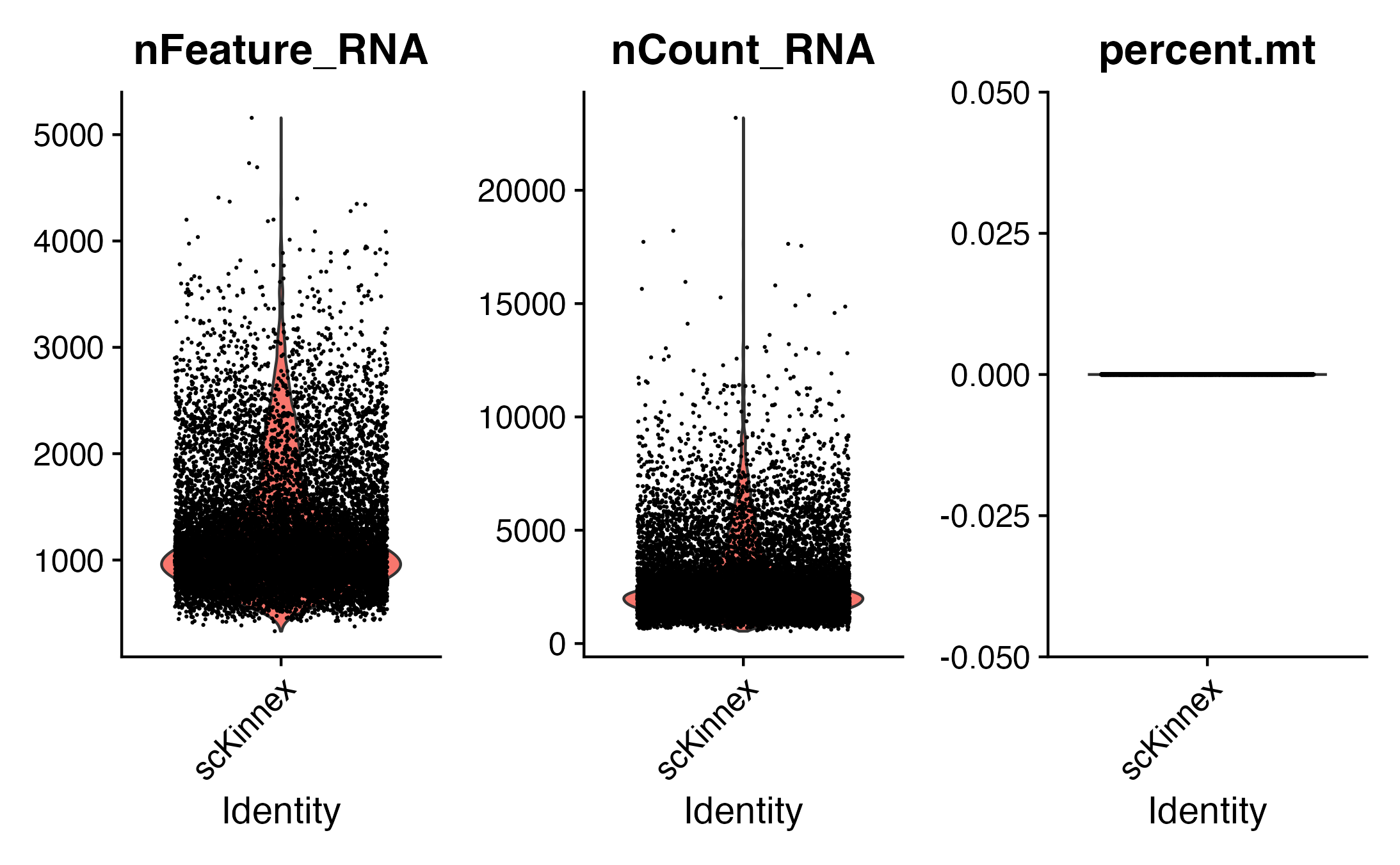
Visualize QC metrics as a violin plot
VlnPlot: Draws a violin plot of single cell data (gene expression, metrics, PC scores, etc.)
#{r}
# Visualize QC metrics as a violin plot
VlnPlot(seurat_obj, features = c("nFeature_RNA", "nCount_RNA", "percent.mt"), ncol = 3)
#{r}
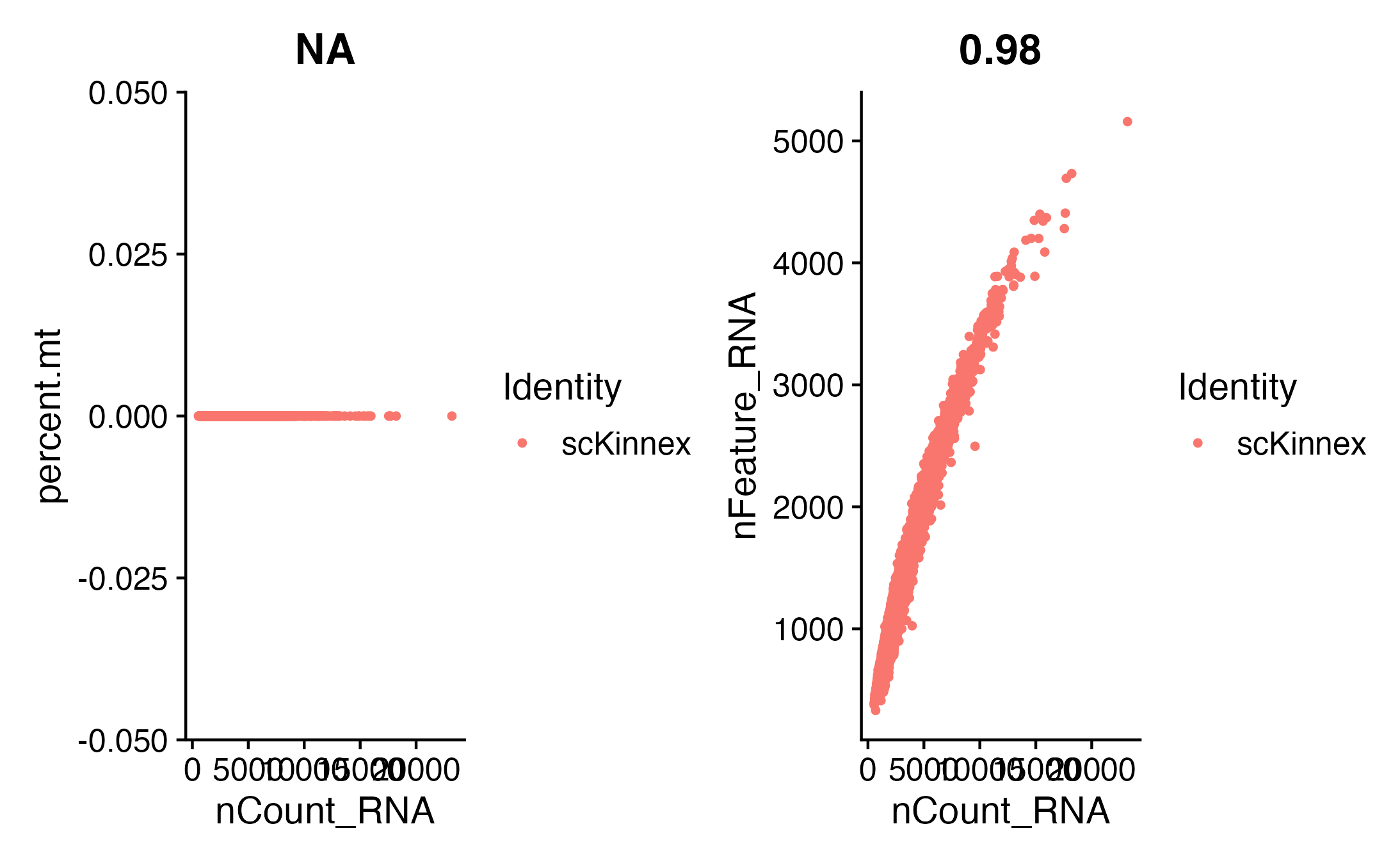
plot1 <- FeatureScatter(seurat_obj, feature1 = "nCount_RNA", feature2 = "percent.mt")
plot2 <- FeatureScatter(seurat_obj, feature1 = "nCount_RNA", feature2 = "nFeature_RNA")
plot1 + plot2
Saving object.RDS
#{r}
#saveRDS(seurat_obj, file = paste0(data_dir, output_prefix, "-seurat_obj-preCellFiltering.rds"))
filtering cells on percent Mitochondria:
#{r}
#### filtering cells on
length(seurat_obj$percent.mt < 15)
seurat_obj <- subset(seurat_obj,
                 percent.mt < 15)
seurat_obj
Terminal Out: An object of class Seurat 25943 features across 12851 samples within 1 assay Active assay: RNA (25943 features, 0 variable features) 1 layer present: counts
Summarize:
#{r}
    seurat_obj@meta.data %>% summarize(median(nCount_RNA), median(nFeature_RNA))
Terminal Output: median(nCount_RNA) median(nFeature_RNA) <dbl> <int> 2250.01 1087
NormalizeData : Normalize the count data present in a given assay. Normalization methods = “LogNormalize”: Feature counts for each cell are divided by the total counts for that cell and multiplied by the scale.factor. This is then natural-log transformed using log1p.
#{r}
seurat_obj <- NormalizeData(seurat_obj, normalization.method = "LogNormalize", scale.factor = 10000)
FindVariableFeatures: Identifies features that are outliers on a ‘mean variability plot’.
selection.method = “vst”: First, fits a line to the relationship of log(variance) and log(mean) using local polynomial regression (loess). Then standardizes the feature values using the observed mean and expected variance (given by the fitted line). Feature variance is then calculated on the standardized values after clipping to a maximum (see clip.max parameter).
#{r}
seurat_obj <- FindVariableFeatures(seurat_obj, selection.method = "vst", nfeatures = 2000)

# Identify the 10 most highly variable genes
top10 <- head(VariableFeatures(seurat_obj), 10)

# plot variable features with and without labels
plot1 <- VariableFeaturePlot(seurat_obj)
plot2 <- LabelPoints(plot = plot1, points = top10, repel = TRUE)
plot1 + plot2
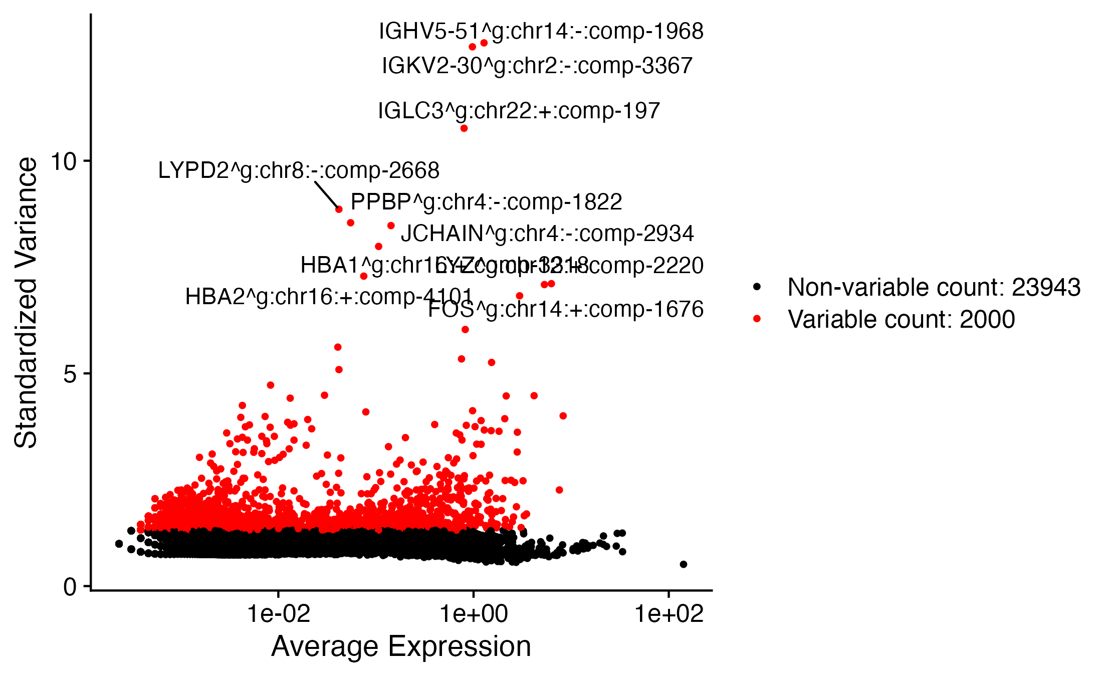
ScaleData: Scales and centers features in the dataset. If variables are provided in vars.to.regress, they are individually regressed against each feature, and the resulting residuals are then scaled and centered.
#{r}
all.features <- rownames(seurat_obj)
seurat_obj <- ScaleData(seurat_obj, features = all.features)
Performing PCA :#
RunPCA: Run Principal Component Analysis on gene expression using IRLBA. For details about stored PCA calculation parameters, see PrintPCAParams.
#{r}
seurat_obj <- RunPCA(seurat_obj, features = VariableFeatures(object = seurat_obj))
VizDimLoadings: Visualize top genes associated with reduction components
#{r}

VizDimLoadings(seurat_obj, dims = 1:2, reduction = "pca")

DimPlot: Graphs the output of a dimensional reduction technique (PCA by default). Cells are colored by their identity class.
#{r}

DimPlot(seurat_obj, reduction = "pca") + NoLegend()
DimHeatmap(seurat_obj, dims = 1:3, cells = 500, balanced = TRUE)
ElbowPlot(seurat_obj)


Generating UMAP :#
#{r}
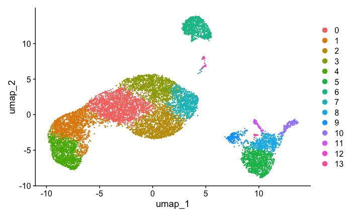
seurat_obj <- FindNeighbors(seurat_obj, dims = 1:8)
seurat_obj <- FindClusters(seurat_obj, resolution = 0.8)
seurat_obj <- RunUMAP(seurat_obj, dims = 1:8)
DimPlot(seurat_obj, reduction = "umap")

FeaturePlot(seurat_obj, features = c("nFeature_RNA"))

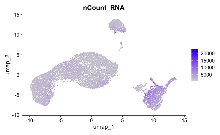
FeaturePlot(seurat_obj, features = c("nCount_RNA"))

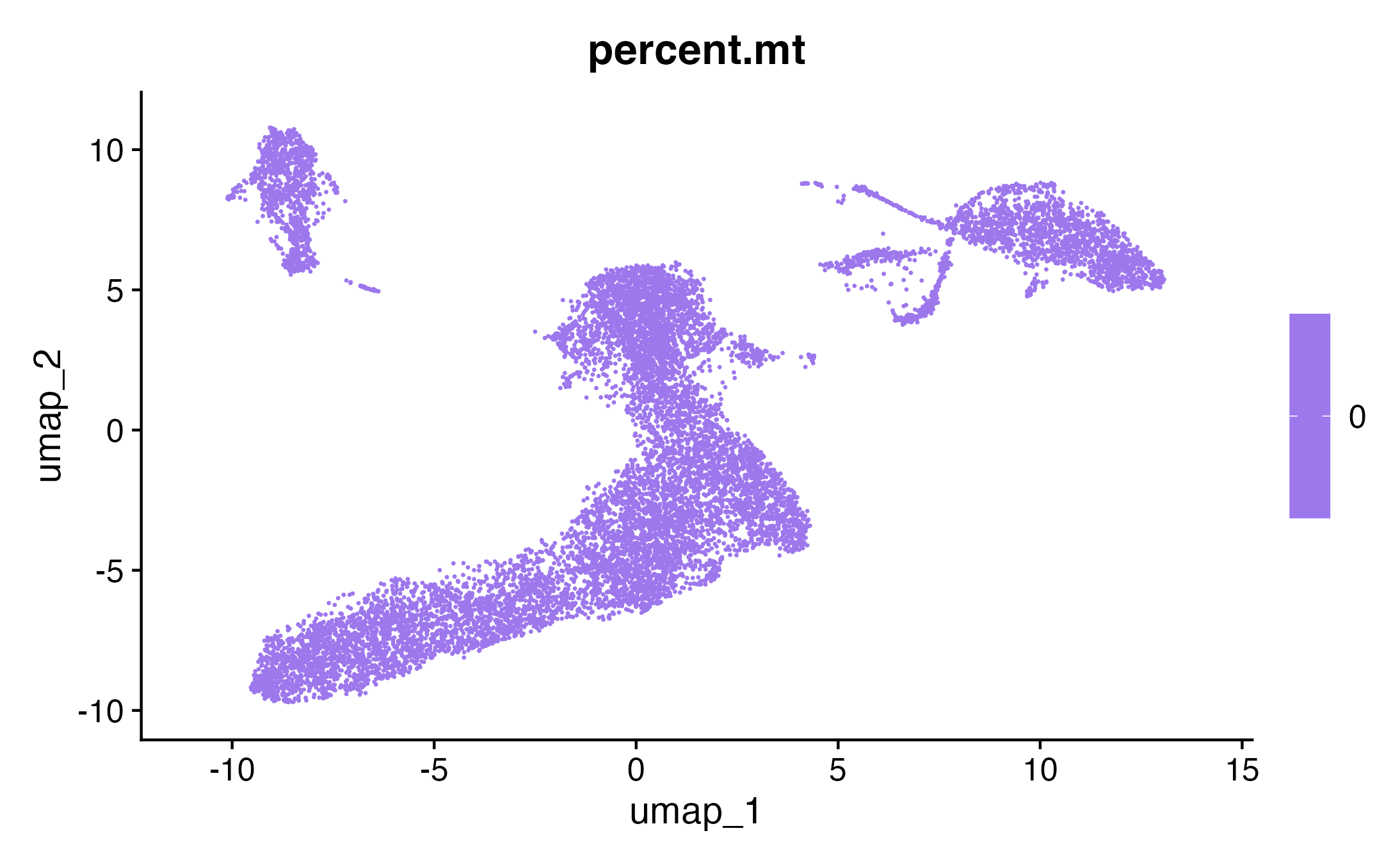
FeaturePlot(seurat_obj, features = c("percent.mt"))
Feature Count plots from terminal out:
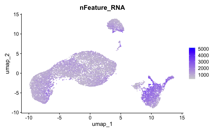
Feature Count plots from terminal out:
#{r}
# counts and fractions of cells

cluster_counts_n_fracs = seurat_obj@meta.data %>% group_by(seurat_clusters) %>% tally() %>%  mutate(frac=prop.table(n))

cluster_counts_n_fracs

saveRDS(seurat_obj, file = paste0(output_prefix, "-seurat_obj.rds"))
Terminal Out:
seurat_clusters n frac <fctr> <int> <dbl> 0 2243 0.174538946 1 1765 0.137343397 2 1693 0.131740721 3 1476 0.114854875 4 1358 0.105672710 5 1112 0.086530231 6 1040 0.080927554 7 979 0.076180842 8 523 0.040697222 9 262 0.020387518 10 218 0.016963660 11 102 0.007937126 12 54 0.004202008 13 26 0.002023189
DE, find markers:#
find markers for every cluster compared to all remaining cells, report only the positive ones
#{r}
# find markers for every cluster compared to all remaining cells, report only the positive
# ones
seurat_obj.markers <- FindAllMarkers(seurat_obj, only.pos = TRUE)
seurat_obj.markers %>%
    group_by(cluster) %>%
    dplyr::filter(avg_log2FC > 1)
#{r}
top_20_markers = seurat_obj.markers %>%
group_by(cluster) %>%
dplyr::filter(avg_log2FC > 1) %>% slice_head(n=20) %>% ungroup()


top_20_markers
#{r}
max_cluster <- max(as.numeric(top_20_markers$cluster)) - 1

for (clnum in 0:max_cluster) {
    cluster = top_20_markers %>% filter(cluster == clnum)


        gene.symbols = sapply(cluster$gene, function(x) { str_split(x, "\\^")[[1]][1] })

        gene.symbols = grep("ENSG|ENST|novel", gene.symbols, value=T, invert=T)

    cat(paste0(clnum,":"))
    cat(gene.symbols, sep=",")
    cat("\n")
}
Terminal Out:

0:LTB,IL7R,RNU1-125P,NOSIP,TNFRSF4,LDHB,AQP3,RGCC,KLRB1,IL7R,GZMK,CD40LG,GPR171,TRADD,CCR4,NPDC1,MAL,IFNG-AS1,CD69
1:NKG7,GZMA,CCL5,LINC00987,A2M,GZMK,RNU1-125P,RNU6-1257P,SAMD3,PZP,TGFBR3,DUSP2,PYHIN1,GZMM,CCL4,KLRD1,GZMH,LINC01871,TRGV3,KLRC1
2:LEF1,CCR7,LINC02446,LRRN3,RPS16,RPS6,MIR7111,RPS3A,RPL19,RPL35A,ARL6IP1,RPL32,RPS28,SNORD38B,RPL34,TPT1,RPS23,RPL13,RPS12,RPS14
3:INPP4B,CDC14A,KLF12,LINC-PINT,ARHGAP15,PAG1,SKAP1,TC2N,CABYR,SERINC5,HIVEP2,STARD4-AS1,ANK3,BCL11B,CDC42SE2,BCL2,CYTH1,HELZ-AS1
4:NKG7,GNLY,GZMA,CCL5,KLRC1,RNU6-1257P,GZMH,KLRD1,TGFBR3,FGFBP2,GZMB,TRGV3,SAMD3,PYHIN1,CCL4,TRDC,GZMM,KLRF1,CX3CR1,HOPX
5:S100A8,MNDA,VCAN,CST3,FCN1,CD36,PLXDC2,TYROBP,RGS2,MS4A6A,CYBB,FOS,FGL2,CD14,LST1,CEBPD,AIF1,LYZ,ODF3B
6:BANK1,IGHV5-51,RALGPS2,AFF3,FCRL1,MS4A1,MEF2C,HLA-DRA,HLA-DPA1,HLA-DQA1,MARCHF1,CD79B,HLA-DMA,CD79A,HLA-DPB1,LYN,STX7,CD74,IGKV2-30,AFF3
7:LEF1,HELZ-AS1,BACH2,FHIT,MAML2,EIF4E3,CYP2R1,STARD4-AS1,TXK,SERINC5,MLLT3,MBNL1,BCL11B,C6orf132,FHIT,PDE7A,IL6ST,ARHGAP15,SATB1
8:MNDA,CST3,FCN1,PLXDC2,FGL2,CD36,LST1,MS4A6A,TYROBP,SPI1,PSAP,IGSF6,VCAN,CYBB,AIF1,HLA-DRA,CPPED1,GPX1
9:PLXDC2,RBM47,VCAN,ZEB2,SLC8A1,LRMDA,LYN,TBXAS1,AOAH,CPPED1,ARHGAP26,DMXL2,GRK3,CD36,MARCHF1,ATG7,NAMPT,DPYD
10:FCGR3A,MS4A14,PELATON,SERPINA1,IFITM3,CSF1R,LILRB2,LRRC25,CLN6,LINC02432,MYOF,CD300H,CTSL,NDUFB9,MS4A4A,HMOX1,LYPD2,CKB,CDKN1C,TCF7L2
11:FCER1A,CD1C,ENHO,CLEC10A,ATP1B1,CLIC2,FLT3,MIR511,PLD4,TIFAB,ZNF366,HLA-DPB2,IL18,CD1E,FCGR2B,TNFSF15
12:MZB1,CLEC4C,DERL3,PTPRS,SCT,PTCRA,PTPRS,LRRC26,SLC35F3,CUX2,PPP1R14B-AS1,SLC12A3,GLDC,SCAMP5,PHEX
13:GPRIN1,FCRL1,ADAM28,BANK1,LINC00926,g:chr1:-:comp-25443,OSBPL10,MS4A1,CD79A,MTARC2,CPNE5,FAM30A,LINC02397,FCGR1A,NMNAT1,PLEKHG1,CD40,COBLL1
using clustermole to add annotations:
#{r}
library(clustermole)
clustermole_results = NULL

for (clnum in 0:max_cluster) {
    cluster = top_20_markers %>% filter(cluster == clnum)

    gene.symbols = sapply(cluster$gene, function(x) { str_split(x, "\\^")[[1]][1] })

    gene.symbols = grep("ENSG|ENST|novel", gene.symbols, value=T, invert=T)


tryCatch(
    expr = {

    cat(paste0(clnum,":"))
    cat(gene.symbols, sep=",")
    cat("\n")

    my_overlaps <- clustermole_overlaps(genes = gene.symbols, species = "hs")

    clustermole_results = bind_rows(
        clustermole_results,
                              my_overlaps %>% mutate(clnum = clnum))
    },
    error = function(e){
    message("Error: ", e)
    },
    warning = function(w){
    message("Warning: ", w)
    }
)
}


clustermole_summary = clustermole_results  %>% filter(db == "PanglaoDB") %>%
group_by(clnum) %>% arrange(p_value) %>% filter(row_number() == 1) %>% arrange(clnum) %>%
ungroup() %>%
dplyr::select(clnum, organ, celltype, fdr)

clustermole_summary
clnum organ celltype fdr <int> <chr> <chr> <dbl> 0 Immune system T cells 1.338613e-03 1 Immune system NK cells 7.001437e-17 2 Immune system T memory cells 2.180756e-02 3 Immune system T memory cells 7.487984e-04 4 Immune system NK cells 1.397130e-25 5 Immune system Macrophages 1.327224e-08 6 Immune system B cells 4.417823e-09 7 Immune system T memory cells 1.208889e-02 8 Immune system Macrophages 8.000349e-09 9 Blood Reticulocytes 2.323308e-01 10 Immune system Dendritic cells 2.491410e-01 11 Immune system Dendritic cells 1.833132e-02 12 Immune system Plasmacytoid dendritic cells 8.752285e-06 13 Immune system B cells naive 1.240425e-06
#{r}
# save files for later read/cell tracking

write.table( Idents(seurat_obj), paste0(output_prefix, "-cell_cluster_assignments.tsv"), quote=F, row.names=T, sep="\t")
#{r}
saveRDS(seurat_obj, file = paste0(output_prefix, "-seurat_obj.rds"))
Installing clustermole: https://cran.rstudio.com/web/packages/clustermole/vignettes/clustermole-intro.html
#{r}
#BiocManager::install("igordot/clustermole", update = FALSE)
Examining specific gene sets example Note, this helps to have the gene-symbol annotated gene features.
#{r}
# example definition of marker genes for certain cell types

marker_genes = list()

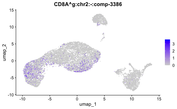
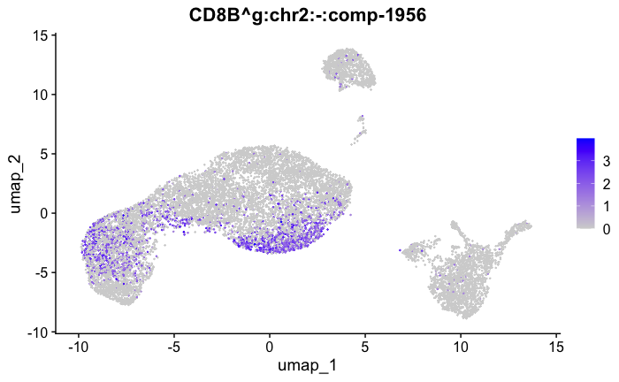
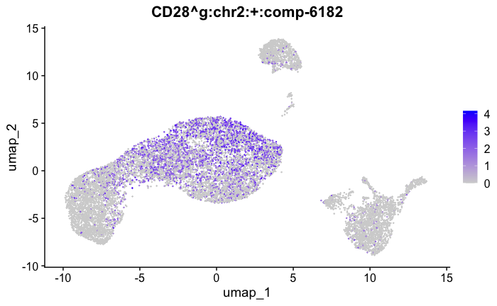
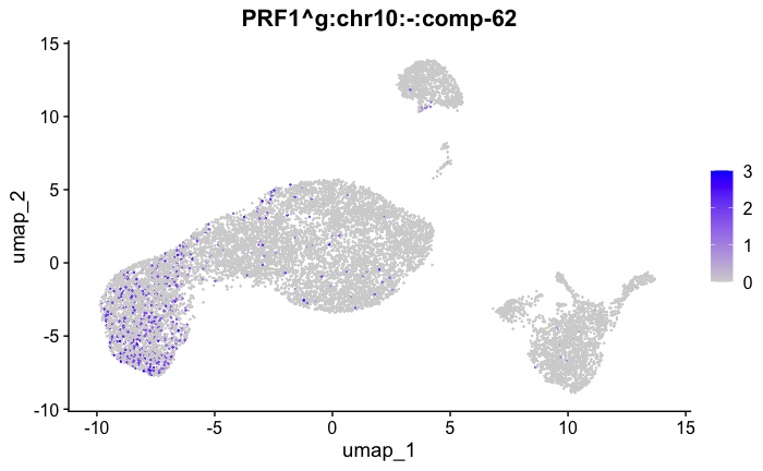
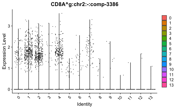
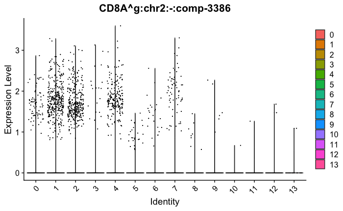
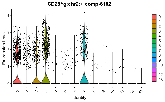
marker_genes[["Tcells"]] = c("CD8A","CD8B","CD3","CD4","CD127","PRF1", "GZMB", "CD28","LTB")
#{r}

# function to extract gene ids with the relevant gene symbols


feature_names = rownames(seurat_obj@assays$RNA$counts)

get_feature_names_with_gene_symbols = function(gene_symbols) {

gene_ids = c()

for (gene_symbol in gene_symbols) {
    found_genes = grep(paste0(gene_symbol,"\\^"), feature_names, value=T)
 if (length(found_genes) > 0) {
        gene_ids = c(gene_ids, found_genes)
    }
}
return(gene_ids)
}
#{r}
# paint umaps according to the features of interest
feature_ids = get_feature_names_with_gene_symbols(marker_genes[["Tcells"]])

VlnPlot(seurat_obj, features = feature_ids, combine=FALSE)
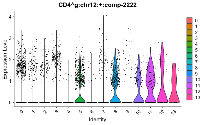

#{r}

FeaturePlot( seurat_obj, features = feature_ids)